The problem attention solves
Consider the sentence "the animal did not cross the street because it was too tired." To process the word "it," a model has to know that "it" refers to the animal, not the street. The information needed to understand one word lives in other words, sometimes far away. The central problem in language modeling is moving the right context to the right place.
The architectures that came before transformers, recurrent networks, did this by reading left to right and carrying a single fixed-size summary of everything seen so far. That summary is a bottleneck. It has to compress the entire past into one vector, and the further back a relevant word is, the more it has faded by the time it is needed. Worse, the reading is sequential, so it cannot be parallelized across positions.
Attention replaces the bottleneck with direct access. Every position can read from every other position in a single step, and it learns which positions to read from. No fixed summary, no distance penalty, fully parallel. That is the whole pitch. The rest of this article is how it actually works.
Query, key, and value
The cleanest way to understand attention is as a soft dictionary lookup. An ordinary dictionary maps a key to a value: you supply a query, find the key that matches exactly, and return its value. Attention does the same thing, except the match is not all-or-nothing. Instead of returning the one value whose key matches, it returns a blend of all values, weighted by how well each key matches the query.
Every token produces three vectors, each by multiplying its embedding by a learned weight matrix:
- Query (\(q\)): what this token is looking for.
- Key (\(k\)): what this token offers, the label others match against.
- Value (\(v\)): the information this token contributes once matched.
The query and key are used only to compute compatibility. The value is what actually gets passed along. Keeping them separate is what gives attention its flexibility: a token can advertise one thing (its key) while contributing another (its value), and what it looks for (its query) is independent of both.
It is tempting to ask why keys and values are different. If a token both matches and contributes, why not use one vector for both? Because the question "is this token relevant to me?" and "what should I take from it?" are genuinely different. The word "bank" might be highly relevant to "river" (strong key match) while the information worth passing along is its sense, not its spelling (a different value). Separating key from value lets the model learn these independently.
A worked example, by hand
Abstract formulas hide where the numbers come from, so let us run a complete example end to end with real values. We will use a three-token sequence, "the cat sat," with a model dimension of 4 and query, key, and value dimensions of 3. Every number below is reproducible from the code at the end of this section.
Start with the token embeddings, one row per token. In a real model these come from the embedding table and earlier layers; here we just fix them:
The model has three learned projection matrices, \(W_Q\), \(W_K\), and \(W_V\), each mapping the 4-dimensional embedding to a 3-dimensional space. Multiplying the embeddings by them produces the query, key, and value matrices, one row per token:
Each row of \(Q\) is one token's query, each row of \(K\) one token's key, each row of \(V\) one token's value. Now we compute attention for all three tokens at once.
Step 1: scores
To find how much a query token should attend to a key token, take the dot product of the query with the key. A large dot product means the two vectors point in similar directions, which the model has learned to interpret as relevance. Doing this for every query against every key is a single matrix multiplication:
Read row by row. The first row, \([2, 8, 6]\), is how much the query for "the" matches the keys for "the," "cat," and "sat." The raw scores already show a pattern: every token scores highest against "cat."
Step 2: scale by √dₖ
Before turning scores into weights, we divide by \(\sqrt{d_k}\), the square root of the key dimension. Here \(d_k = 3\), so we divide by \(\sqrt{3} \approx 1.73\):
This step looks fussy but it matters. The dot product of two vectors with \(d_k\) independent components, each of roughly unit variance, has variance proportional to \(d_k\). As \(d_k\) grows, raw scores grow with it, and large scores push the softmax in the next step into a regime where it returns almost all of its weight to a single token and almost nothing to the rest. In that regime the gradient nearly vanishes and learning stalls. Dividing by \(\sqrt{d_k}\) cancels the growth and keeps the scores in a range the softmax handles gracefully.
If \(q\) and \(k\) have components that are independent with mean 0 and variance 1, then \(q \cdot k = \sum_{i=1}^{d_k} q_i k_i\) has mean 0 and variance \(d_k\). Standard deviation therefore scales as \(\sqrt{d_k}\). Dividing the dot product by \(\sqrt{d_k}\) restores unit variance regardless of dimension, which is exactly what keeps the softmax well-behaved as models scale their head dimension up.
Step 3: softmax
Now convert each row of scaled scores into a probability distribution with the softmax function, which exponentiates each value and normalizes so the row sums to one:
Applied row by row, this gives the attention weights: for each query token, how much of its attention goes to each key token.
Every row sums to 1, so each query token spreads exactly one unit of attention across the sequence. The pattern the raw scores hinted at is now explicit: all three tokens attend most strongly to "cat." This is a toy example, but it shows the mechanism. In a trained model these weights encode real linguistic structure, such as a pronoun concentrating its weight on the noun it refers to.
Step 4: the weighted sum
Finally, each token's output is the weighted sum of all value vectors, using its attention weights. This is one more matrix multiplication, \(A\) times \(V\):
Each row is a new representation of the corresponding token, built by pulling in information from the tokens it attended to. Because all three tokens attended mostly to "cat," all three outputs look similar to "cat"'s value vector \([2, 8, 0]\), nudged by the smaller contributions from the others. The token has, in a real sense, gathered its context.
The whole thing in NumPy
import numpy as np

X  = np.array([[1,0,1,0],[0,2,0,2],[1,1,1,1]], dtype=float)   # 3 tokens, d_model=4
Wq = np.array([[1,0,1],[1,0,0],[0,0,1],[0,1,1]], dtype=float)  # 4 x 3
Wk = np.array([[0,1,1],[1,1,0],[0,1,0],[1,0,1]], dtype=float)
Wv = np.array([[0,2,0],[0,3,0],[1,0,3],[1,1,0]], dtype=float)

Q, K, V = X @ Wq, X @ Wk, X @ Wv
dk = Q.shape[1]

scores = Q @ K.T / np.sqrt(dk)
weights = np.exp(scores - scores.max(1, keepdims=True))
weights /= weights.sum(1, keepdims=True)        # softmax over each row
output = weights @ V

print(weights.round(2))   # [[0.02 0.74 0.23] [0. 0.76 0.24] [0. 0.85 0.15]]
print(output.round(2))    # [[1.98 7.39 0.77] [2. 7.51 0.72] [2. 7.69 0.45]]
The complete formula
Everything above collapses into the single equation from Attention Is All You Need [1]:
Now every symbol has a meaning you derived. \(QK^\top\) scores every query against every key. \(\sqrt{d_k}\) keeps those scores well-scaled. The softmax turns them into weights that sum to one. Multiplying by \(V\) takes the weighted sum of values. This is called scaled dot-product attention, and it is the entire operation. Everything else in a transformer is built around it.
Multi-head attention
A single attention operation learns one notion of relevance. But language has many relationships at play simultaneously: subject and verb agreement, what a pronoun refers to, topic, sentiment. Forcing all of them through one set of \(Q\), \(K\), \(V\) projections is limiting.
Multi-head attention runs several attention operations in parallel, each with its own learned projections, so each head can specialize. With \(h\) heads, the model dimension \(d_{\text{model}}\) is split into \(h\) pieces of size \(d_k = d_{\text{model}} / h\). Each head computes scaled dot-product attention in its own subspace, the outputs are concatenated back to full width, and a final projection \(W_O\) mixes them:
The cost is roughly the same as a single full-width head, because each head works in a smaller subspace. The benefit is that one head can track verb agreement while another tracks coreference, and the model is not forced to compromise between them. In practice, inspecting trained heads shows exactly this kind of specialization.
Causal masking
A model like GPT or Claude generates text left to right, predicting the next token from the ones before it. During training, it sees whole sequences at once, which creates a problem: when learning to predict token 3, it must not be allowed to attend to tokens 4 and beyond, or it would simply copy the answer.
The fix is a causal mask. Before the softmax, every score where a query attends to a future key is set to \(-\infty\) (in practice a large negative number). After the softmax, those positions become exactly zero. Applied to our example, the lower-triangular structure appears:
"the" can only attend to itself, "cat" to "the" and "cat," "sat" to all three. Information flows only backward in time, which is exactly what next-token prediction requires. This single change is the difference between an encoder (bidirectional, like BERT) and a decoder (causal, like GPT).
The cost of attention
Attention's power, every position seeing every other, is also its expense. For a sequence of length \(n\), the score matrix \(QK^\top\) has \(n^2\) entries, so both compute and memory grow with the square of the sequence length. Double the context and attention's cost roughly quadruples.
This single fact drives an enormous amount of LLM engineering. At training time it motivates efficient and approximate attention. At inference time it motivates the KV cache, which avoids recomputing keys and values for past tokens, and the attention variants below, which shrink how much must be stored. Long-context models live or die on how well they manage this quadratic cost, and it is a large part of what our lab's research works on.
Attention variants
Most production attention is not the plain multi-head version. The dominant variants trade a little expressiveness for large savings in the memory the KV cache consumes, by sharing keys and values across query heads.
| Variant | Query heads | Key/value heads | KV cache size | Used by |
|---|---|---|---|---|
| MHA | h | h | Largest | Original transformer, GPT-2 |
| GQA | h | g (groups, 1 < g < h) | Medium | LLaMA 2/3, most modern models |
| MQA | h | 1 | Smallest | PaLM, Falcon |
In multi-query attention all query heads share a single key and value head, shrinking the KV cache by a factor of \(h\) at some cost to quality. Grouped-query attention is the compromise that most current models settle on: a handful of key/value heads shared among groups of query heads, capturing most of the memory saving with little quality loss.
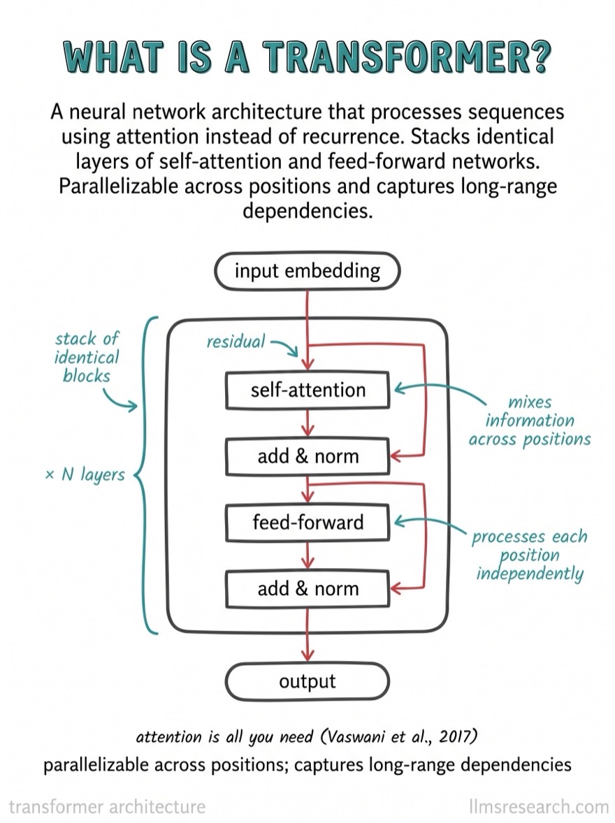
The whole stack, drawn out
This is one concept. The LLM Flashcards cover attention variants, the KV cache, positional encoding, training, RAG, and the rest in 376 visual cards, as a PDF and an Anki set.
See the cards →Review the ideas as visual cards
References
- Vaswani et al. Attention Is All You Need. NeurIPS, 2017. The paper that introduced scaled dot-product and multi-head attention.
- Shazeer. Fast Transformer Decoding: One Write-Head is All You Need. 2019. Multi-query attention.
- Ainslie et al. GQA: Training Generalized Multi-Query Transformer Models from Multi-Head Checkpoints. 2023. Grouped-query attention.