What came before, and why it broke
Until 2017, the standard tool for language was the recurrent neural network and its variants like the LSTM. These read a sequence one token at a time, maintaining a hidden state that summarized everything seen so far. Two limits held them back. They were inherently sequential, so token \(t\) could not be processed until token \(t-1\) was done, which wasted the parallel hardware that makes deep learning practical. And the single hidden state was a bottleneck: information from early tokens degraded as it was repeatedly overwritten, so long-range dependencies were fragile.
The transformer, introduced in Attention Is All You Need [1], removed both limits at once by replacing recurrence with attention. Every position is processed in parallel, and every position can read directly from every other, regardless of distance. That is the whole idea. What follows is how the architecture turns that idea into a working model.
A transformer from a distance
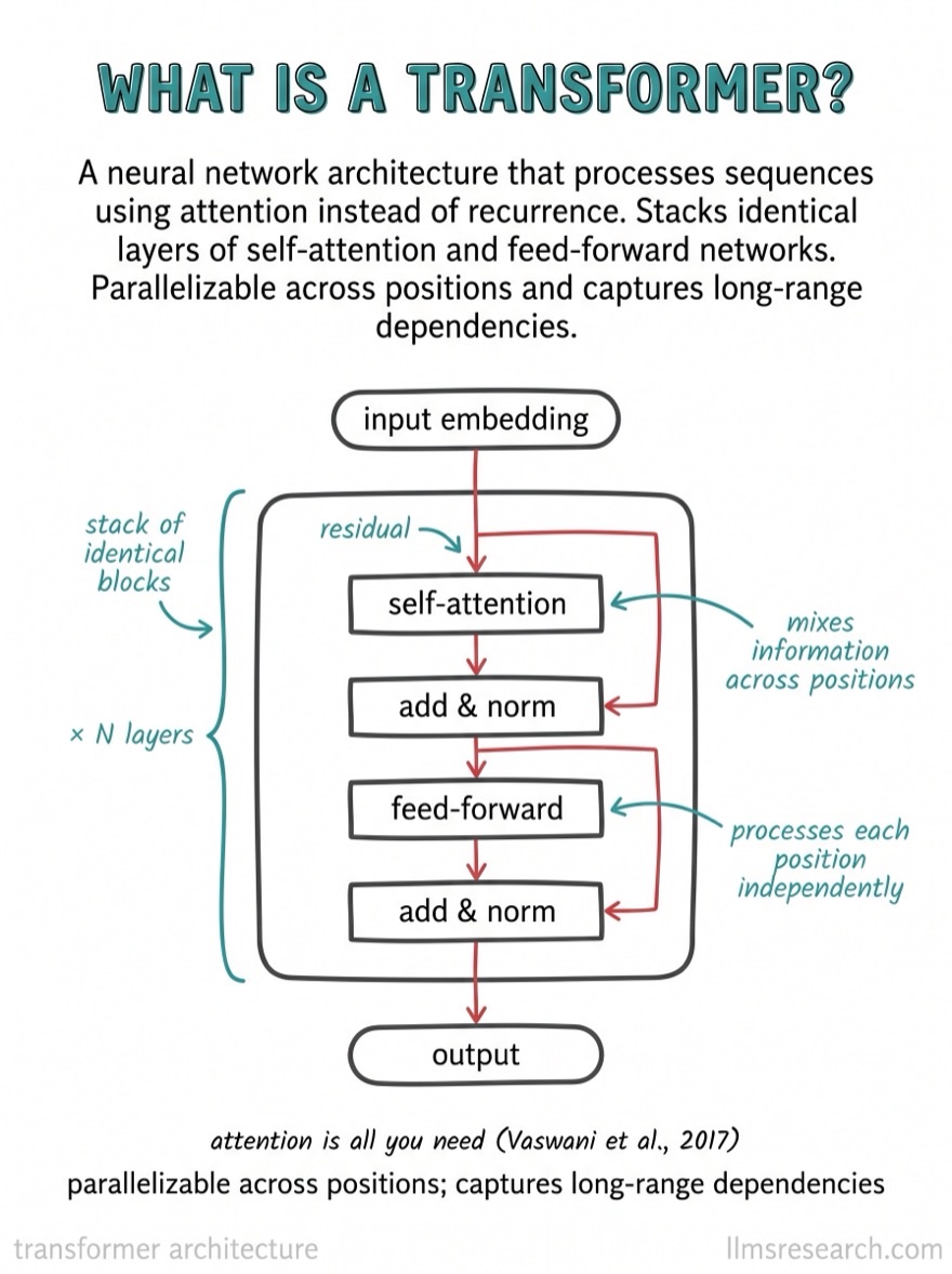
At the highest level, a transformer is a stack of identical blocks. Text enters as a sequence of tokens, gets turned into vectors, flows up through the stack, and exits as a prediction. Each block does the same two things: it lets positions exchange information (attention), then processes each position on its own (a small neural network). Everything else is plumbing that makes those two operations trainable at depth.
A modern model might stack 32, 80, or more of these blocks. The block is the unit worth understanding deeply, because once you know one block, you know the model. Here is the anatomy we will build:
Tokens to vectors
A model does not operate on text. The first step, tokenization aside, is to map each token to a vector. The model holds an embedding matrix \(E \in \mathbb{R}^{V \times d}\), where \(V\) is the vocabulary size and \(d\) is the model dimension. Each token id selects one row, a learned \(d\)-dimensional vector. A sequence of \(n\) tokens becomes a matrix \(X \in \mathbb{R}^{n \times d}\).
These vectors are learned during training, and they arrange themselves so that tokens used in similar ways end up near each other in the space. That geometry is the raw material attention then operates on.
Positional encoding
Attention has a curious blind spot: it is permutation invariant. Because every position attends to every other with no built-in sense of order, "dog bites man" and "man bites dog" would look identical to a bare attention layer. The model has to be told where each token sits.
The original transformer adds a positional encoding to each embedding, a vector that depends only on position. The paper uses fixed sinusoids of geometrically increasing wavelength:
Each dimension is a sine or cosine of a different frequency, so the combination gives every position a unique, smooth signature the model can read. Modern models often replace this with rotary position embeddings (RoPE), which encode relative position by rotating the query and key vectors, but the purpose is the same: inject order into an order-blind mechanism.
The attention sublayer
The first operation in every block is multi-head self-attention. Each token forms a query, every token forms a key and a value, and each token's output is a weighted sum of all values, where the weights come from how well its query matches each key. This is the mechanism that moves context between positions, and it is worth understanding in full detail on its own.
We work attention out from scratch, with a complete numerical example, in How attention works in LLMs. For this guide it is enough to know that the attention sublayer takes \(X \in \mathbb{R}^{n \times d}\) and returns a same-shaped matrix in which each token has gathered information from the tokens it attended to.
Residuals and layer normalization
Two supporting pieces wrap each sublayer, and without them deep transformers do not train. The first is the residual connection: the block adds a sublayer's input back to its output.
This sounds trivial and is profound. Stacking dozens of nonlinear layers normally causes the training gradient to vanish or explode as it propagates back through them. The residual gives the gradient a direct path from the top of the network to the bottom, bypassing every sublayer if needed. It is the single change that made very deep networks trainable, and the transformer relies on it at every sublayer.
The second is layer normalization, which rescales each token's vector to zero mean and unit variance, then applies a learned scale \(\gamma\) and shift \(\beta\):
where \(\mu\) and \(\sigma^2\) are the mean and variance across the vector's \(d\) components. This keeps activations in a stable range as they pass through many layers. Where exactly the norm is placed matters: the original transformer applied it after the residual add (post-norm), but nearly all modern models apply it before the sublayer (pre-norm), because pre-norm is markedly more stable to train at depth.
The feed-forward sublayer
After attention has mixed information across positions, each token is processed independently by a small two-layer network, the same network applied to every position. It expands the vector to a larger inner dimension (classically \(4d\)), applies a nonlinearity, and projects back down:
If attention decides what to look at, the feed-forward network decides what to do with it. It is also where most of a transformer's parameters live. With inner dimension \(4d\), the two matrices hold \(8d^2\) parameters per block, against roughly \(4d^2\) for the four attention projections. The part of the model people talk least about holds two thirds of its weights.
For a model with \(d = 4096\): each block has about \(4d^2 \approx 67\text{M}\) attention parameters and \(8d^2 \approx 134\text{M}\) feed-forward parameters, roughly \(200\text{M}\) per block. Across 32 blocks plus embeddings, that lands near 7 billion, which is exactly the size of a "7B" model. The names are not arbitrary.
One block, end to end
Putting the pieces in order, here is what one pre-norm block does to its input \(x\):
Two sublayers, each wrapped in a norm and a residual. Notice the shape never changes. The input is \(n \times d\), every intermediate is \(n \times d\), and the output is \(n \times d\). That shape invariance is what lets the blocks stack: the output of one is a valid input to the next.
| Stage | Shape | What changed |
|---|---|---|
| Input x | n × d | token vectors entering the block |
| After attention + residual | n × d | each token has gathered context |
| After FFN + residual | n × d | each token processed independently |
| Block output | n × d | ready for the next block |
Stacking blocks
A single block performs one round of "look around, then think." Stacking \(N\) of them lets representations grow richer with depth. Probing trained models shows a rough progression: lower blocks capture surface features like part of speech and local syntax, middle blocks capture phrase and clause structure, and upper blocks capture meaning, reference, and task-relevant abstractions. Depth is not redundant repetition; each block refines what the ones below produced.
Encoder, decoder, encoder-decoder
The same block comes in three arrangements, and the difference is mostly about which tokens attention is allowed to see.
| Family | Attention | Trained to | Example | Best at |
|---|---|---|---|---|
| Encoder-only | Bidirectional | Fill in masked tokens | BERT | Understanding: classification, retrieval |
| Decoder-only | Causal (past only) | Predict the next token | GPT, Claude, LLaMA | Generation |
| Encoder-decoder | Both, plus cross-attention | Map input to output sequence | T5, original transformer | Translation, summarization |
Modern general-purpose LLMs are almost all decoder-only. The causal mask, which prevents a token from attending to future tokens, is what makes next-token prediction a well-posed training objective: the model can never peek at the answer it is trying to predict.
From block to prediction
After the final block, each token's vector is mapped back to vocabulary space by an output projection, producing a logit for every token in the vocabulary. A softmax turns those logits into a probability distribution over the next token:
Training maximizes the probability the model assigns to the actual next token across an enormous amount of text. That single, simple objective, applied at scale, is what produces everything from grammar to reasoning. The architecture's job is to make that objective learnable; the capability emerges from the data.
Why it took over
Within eighteen months of the 2017 paper, essentially every serious NLP system was rebuilt on transformers. The reason was not a single task improving. It was that one architecture, scaled up and trained on enough text, did nearly every language task well, and kept improving predictably as it was made larger. That reliability, captured later in the scaling laws, turned "make it bigger" into a strategy rather than a gamble. GPT, BERT, T5, LLaMA, Claude, Gemini: different recipes, the same block you just built.
The whole stack, one card at a time
This guide is one topic. The LLM Flashcards cover attention variants, normalization, positional encoding, training, RAG, agents, and inference in 330+ visual cards, as a PDF and an Anki set.
See the cards →References
- Vaswani et al. Attention Is All You Need. NeurIPS, 2017.
- Ba, Kiros, Hinton. Layer Normalization. 2016.
- Devlin et al. BERT: Pre-training of Deep Bidirectional Transformers. 2018.
- Su et al. RoFormer: Enhanced Transformer with Rotary Position Embedding. 2021.